Binomial Distribution
Binomial Distribution
Binomial Distribution is a Discrete Distribution.
It describes the outcome of binary scenarios, e.g. toss of a coin, it will either be head or tails.
It has three parameters:
n - number of trials.
p - probability of occurence of each trial (e.g. for toss of a coin 0.5 each).
size - The shape of the returned array.
Discrete Distribution:The distribution is defined at separate set of events, e.g. a coin toss's result is discrete as it can be only head or tails whereas height of people is continuous as it can be 170, 170.1, 170.11 and so on.
Example
Given 10 trials for coin toss generate 10 data points:
from numpy import random
x = random.binomial(n=10, p=0.5, size=10)
print(x)
Try it Yourself »
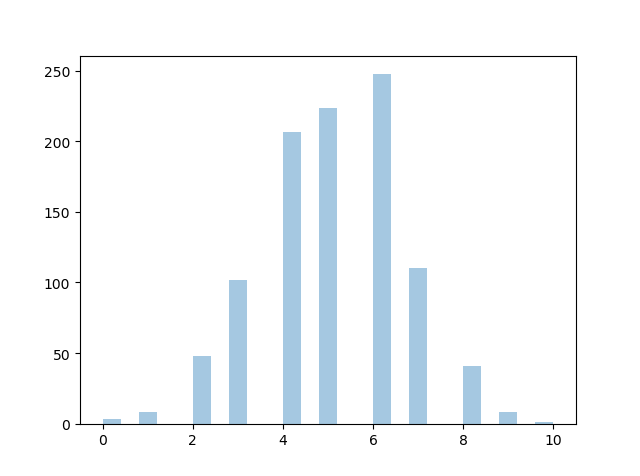
Visualization of Binomial Distribution
Example
from numpy import random
import matplotlib.pyplot as plt
import seaborn as sns
sns.distplot(random.binomial(n=10, p=0.5, size=1000), hist=True, kde=False)
plt.show()
Result
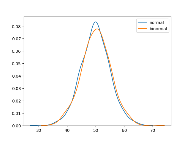
Difference Between Normal and Binomial Distribution
The main difference is that normal distribution is continous whereas binomial is discrete, but if there are enough data points it will be quite similar to normal distribution with certain loc and scale.
Example
from numpy import random
import matplotlib.pyplot as plt
import seaborn as sns
sns.distplot(random.normal(loc=50, scale=5, size=1000), hist=False,
label='normal')
sns.distplot(random.binomial(n=100, p=0.5, size=1000), hist=False,
label='binomial')
plt.show()
Result